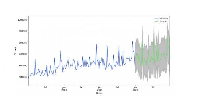
Which statistical methods are helpful for forecasting sales?

Sales data, like the date and quantity of items sold, are one the most valuable data we can use to forecast sales and optimize the supply chain and inventory. If we consider our data as a timeseries, these statistical tools can help us to do the forecasting.
What are time series?
A collection of data points gathered over time is known as a time series. Numerous disciplines, including economics, finance, meteorology, and many more, use time series data.
Regular intervals, such as daily, hourly, or minute-by-minute, are frequently used to collect time series data. This enables the detection and analysis of trends and patterns across time. Additional factors in time series data, such as temperature or humidity, may also be important for the study.
Ok, after we had a brief introduction of timeseries, we will take a look at our interesting tools that can help us to earn more money and obtain a data-driven decision-making approach.
As we already mentioned, time series forecasting is the process of using a model to anticipate future values based on values that have already been observed. Numerous industries, including meteorology, banking, and economics, can benefit from time series forecasting. For time series forecasting, a variety of techniques are available, such as:
- Simple moving average (SMA): The SMA is a simple and effective way to smooth out short-term fluctuations in a time series and identify longer-term trends. It is possible to predict future values by averaging a group of observations over a certain period of time.
For instance, if you have a time series with the following values: 10, 12, 15, 14, 16, 18, 20, 22, 25, 28, and you want to calculate a 10-day SMA, you would add up the values for the first ten days (10+12+15+14+16+18+20+22+25+28) and divide by 10 to get an SMA of 19.
It is often used in conjunction with other forecasting methods to improve the accuracy of predictions. - Exponential smoothing: This technique includes giving previous observations weights that decrease exponentially. Older observations are given progressively lower weights, while the most current observations are given the greatest weights. The concept is similar to SMA, but a few steps need to be added to the latter.
After choosing the time frame (TF), the weighting multiplier (WM) should be calculated with the following formula: WM = 2/(TF+1)
For instance, for 10-days EMA, WM = 2/(10+1) = 0.18
Now it’s time to calculate the EMA amount with the latter coefficient. Let’s assume that the current value is 15 and the EMA for the previous period is 10. Here is the calculation:
EMA = (15 * 0.1818) + (10 * (1 – 0.1818)) = 2.727 + 8.182 = 10.909 - Autoregressive integrated moving average (ARIMA) is a statistical model used for time series forecasting. It is a generalization of the popular autoregressive moving average (ARMA) model and is particularly useful for forecasting time series data that exhibit trends or seasonality.
ARIMA models are based on the idea that a time series can be decomposed into three components: trend, seasonality, and noise. The trend component represents the underlying pattern in the data, while the seasonality component represents repeating patterns over a specific time period (such as monthly or quarterly). The noise component represents the remaining random variations in the data. The calculation and the modelling can be done with R and Python. - Seasonal decomposition: With this approach, a time series is deconstructed into its trend, seasonality, and residual components. Understanding the fundamental causes of a time series and identifying patterns.
The data pattern that underlies a time series, such as an upward or downward trend, is represented by the trend component. The repeated patterns over a predetermined time period, such as monthly or quarterly patterns, are represented by the seasonality component. The remaining random variations in the data that cannot be accounted for by trend or seasonality are represented by the residual component.
Several methods can be used for seasonal decomposition, such as additive, multiplicative and STL methods. - Machine learning methods: A number of machine learning techniques, including support vector machines, decision trees, and linear regression, may be employed for time series forecasting. These techniques can be helpful for dealing with more complicated time series and for adding other factors that could be essential for predicting. We concisely take a look at linear regression.
Linear Regression: It entails fitting a linear equation to the data so that predictions of future values can be made. The foundation of linear regression is the hypothesis that the predictor variable—the variable used to make predictions—and the response variable have a linear relationship (the variable being predicted).
Forecasting time series data with a linear trend can be done using the comparatively straightforward method of linear regression. When predicting time series data with more intricate patterns or relationships, it might not be as successful. It is important to consider variables that are behaving under a controlled situation, and other external variables do not influence them. Last but not least, do not mistake linear regression for correlation.
In general, the individual properties of the time series and the forecast’s objectives will determine the approach for time series forecasting. To choose the optimal strategy, it might be helpful to test out a few alternative ones and compare the outcomes.
